
This post replaces the model in the September 22 bowed-string post. That voice was an extended Karplus-Strong loop with regenerative sustain. It had no friction law, no bridge and no body, and the post said so. The voice described here is a different program: four delay lines per string, a bow that grips through a rosin friction curve, and a body whose motion is fed back into every string.
The instrument plays from MIDI in Entropy's DAW. It also runs offline with no audio device, which is how every number below was produced. Nobody listened to it while it was built, and I make no claim here about how it sounds. What I can claim is what the tests measure.
Environment
- Engine commit
5b84b6b, with the working-tree changes listed in the frontmatter. There is no tag yet, so a reader cloning the public repository cannot reproduce this exact state today. - Rust 1.94.1, edition 2024,
--releasefor everything. Every timing line the report tests print starts withprofile: release. - Windows 11 Pro 10.0.26200, Intel Core i5-12500. Sample rate 44.1 kHz; the strings and coupled body modes run at 88.2 kHz internally.
- Tests and reports are offline. The view pictures are CPU-rasterized by the headless test harness. The live DAW run used the real window and the default output device; I did not record which wgpu backend it picked.
Commands, all from entropy-engine/:
cargo test --release --lib physmod
cargo test --release --test physmod_synth_bdd
cargo test --release --test physmod_view
cargo test --release --test physmod_no_alloc
cargo test --release --test daw_physmod_live
cargo test --release --lib physmod::tests::strings_tuning_report -- --ignored --nocapture
The strings_*_report tests in src/audio/physmod/tests.rs print every measurement quoted below and write the two plots. From examples/studio-bundle/: npx vitest run tests/daw_physmod.test.ts.
Contents
- The model in one chain
- The string
- The bow
- Schelleng's window, measured against the textbook
- The body
- The virtual player
- The instrument laboratory
- Physics View and one held note
- In the DAW
- How this was verified without listening
- Decision log
- Failure notes and known limits
1. The model in one chain
Player, bow, string, bridge, body, output. Each arrow is code:
| Piece | File | Job |
|---|---|---|
| Delay line, filters | dsp.rs | Cubic-Lagrange fractional delay, one-pole and allpass sections, half-band decimator |
| String | string.rs | Four delay lines split at the bow, terminations, stiffness |
| Bow | friction.rs | Friction solved against the string each sample |
| Body | body.rs | 10 coupled modes that move the bridge, 40 radiating modes that colour the output |
| Instrument and player | engine.rs | Up to four bowed strings and six sympathetic ones, one player per string |
| Measurement | analysis.rs | Pitch in cents, level, centroid, harmonics, bow regime, attack time |
| Runtime | mod.rs | PhysModShared for the view, PhysModVoice, PhysModInstrumentVoice, offline rendering |
analysis.rs matters more than its size suggests. The tests, the Entropy.PhysMod.analyzeNote op and the DAW's AI tool all call the same functions, so a claim and its check are one computation.
The old model lived in one file, src/audio/physmod.rs. It is now the directory src/audio/physmod/.
2. The string
The string follows the digital waveguide layout in Julius Smith's Physical Audio Signal Processing: the bow splits the string into two segments, each carrying a velocity wave in both directions, and the string's velocity at the bow is the sum of the two waves arriving there. Smith describes the nut as reflecting velocity waves with a sign inversion, and the bridge the same way with extra losses from its finite driving-point impedance. That is what string.rs builds.
   finger/nut           bow                        bridge
      |  --- a_r --->    |   --- b_r --->            |
      |  <--- a_l ---    |   <--- b_l ---            |
Every sample, the waves arriving at each end reflect. At the bow, the two arriving waves sum to the string's free velocity v_h. The friction solve turns that into the contact velocity v, and the difference is launched both ways:
let v_h = a_r_out + b_l_out;
let (mut v, mut contact) = friction::solve(v_h, ex.bow_velocity, z, ex.bow_force, &self.friction, self.contact);
// ...
let dv = (v - v_h) + ex.external_force / two_z;
// ...
self.a_r.push(finger_ref);
self.a_l.push(b_l_out + dv);
self.b_r.push(a_r_out + dv);
self.b_l.push(bridge_ref);
The four segment lengths plus the phase delay of the termination filters add up to one period. Retuning solves for that sum, so the free string's pitch does not depend on the note, the loss setting or the stiffness (the source comment says within about a cent; I measured bowed notes only, below). Fractional delays use 4-point Lagrange interpolation. A linearly interpolated delay is also a low-pass whose cutoff moves with the fractional part, which turns into note-dependent brightness and breathing under vibrato.
Loss is set per note. The per-trip gain is chosen for a target t60 at the fundamental, split between the bridge and the finger or nut. A fingertip is a softer, lossier termination than the nut (7 kHz against 9 kHz one-pole cutoff, 0.997 against 0.999 gain), and the nut is not lossless. The source comment on that is worth repeating: with a perfectly rigid nut the open strings' Helmholtz motion was measurably fragile.
Stiffness is a cascade of eight first-order allpasses in the loop. A negative coefficient delays low frequencies more than high ones, so upper partials come round sooner and land sharp. The coefficient is found by bisection for a target inharmonicity B, where partial n sits at n f0 sqrt(1 + B n^2).
Evidence: pitch
strings_tuning_report plays each note bowed, at the default bow settings with vibrato and grit off, and measures the fundamental by autocorrelation.
| Instrument | Notes | Worst error |
|---|---|---|
| Violin (body size 0) | 11 notes, G3 to G6 | +2.7 cents (E5) |
| Cello (size 0.72) | 7 notes, C2 to E4 | +1.0 cent |
| Bass (size 1.0) | 6 notes, E1 to D3 | +4.7 cents (G1, 49 Hz) |
The suite's assertions are looser (6 cents violin, 8 cello, 10 bass), so the code sits inside them with room. The cost is at the bottom of the range. E1 (41.2 Hz) takes 0.58 s to settle into one release per period and G1 0.59 s; cello C2 takes 0.20 s; every violin note takes under 50 ms.
Stiffness works, with a ceiling. On a 220 Hz string the eighth partial follows theory to four decimals up to stiffness 0.6:
| Stiffness | Measured, partial 8 over 8 f1 | Theory |
|---|---|---|
| 0.2 | 1.0050 | 1.0050 |
| 0.4 | 1.0199 | 1.0199 |
| 0.6 | 1.0443 | 1.0443 |
| 0.8 | 1.0638 | 1.0774 |
| 1.0 | 1.0638 | 1.1185 |
The solver refuses to let the allpasses' own delay exceed half a period, so on low notes the coefficient stops moving early. At 110 Hz the eighth partial stops at 1.0092 from stiffness 0.4 upward, where theory says 1.0199 at 0.4 and 1.1185 at 1.0. The knob's top setting is a thin metal bar on a high note and a much milder string on a low one. That is in the limits section as well.
3. The bow
friction.rs is the McIntyre, Schumacher and Woodhouse formulation (JASA 74, 1983), with the hyperbolic curve and hysteresis rule from Woodhouse's thermal-friction paper (Acta Acustica 89, 2003). At the contact the string, left alone, would move at v_h. The bow applies a friction force f, which launches f / 2Z both ways (Z is the string's characteristic impedance), so the contact moves at v = v_h + f / 2Z. Friction is capped by the bow force times a coefficient that falls from static toward dynamic as the relative speed grows:
mu(dv) = mu_d + (mu_s - mu_d) * v0 / (v0 + |dv|)The string sticks whenever the force needed to hold it, 2Z |v_b - v_h|, is within mu_s F_b. Otherwise it slips, at the v where the straight line f = 2Z (v - v_h) meets the curve. For this curve that intersection is a quadratic, so there is no iteration:
// (dh - dv)(v0 + dv) = k (mu_d (v0 + dv) + (mu_s - mu_d) v0)
// => dv^2 - b dv - v0 (dh - k mu_s) = 0,  b = dh - v0 - k mu_d
let b = dh - c.v0 - k * c.mu_d;
let disc = b * b + 4.0 * c.v0 * (dh - k * c.mu_s);
Where both a stick and a slip solution exist, the contact keeps doing what it was doing. That hysteresis is what makes the release into slip sharp. The source comment says nothing here is tuned by ear: force is in newtons, speed in m/s, impedance in kg/s. The default rosin is mu_s 0.8, mu_d 0.3, v0 0.1 m/s, the figures Woodhouse uses for his hyperbolic fit; the engine's rosin knob at 0.5 gives v0 0.11.
I did not run the thermal model. The friction here is the older, speed-only curve. Woodhouse's paper reports that the thermal model establishes Helmholtz motion more reliably and more quickly, which is a difference I have not tested.
Evidence: three regimes
The figure is one D4 (293.66 Hz), held, four periods each, taken 0.6 s into the note. The left column is the string's velocity at the bow. The right is the force on the bridge.
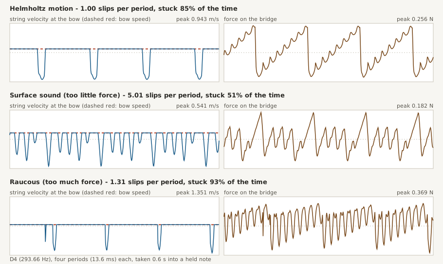
Top row: bow position 0.13 of the string length from the bridge, force knob 0.5, speed knob 0.5 (0.129 m/s). One release per period (1.00 slips per period), stuck 85% of the time against 1 - beta = 0.87. The velocity waveform is what Helmholtz motion predicts: the string rides with the bow, then slips once, quickly, while the corner travels back.
Middle row: position 0.05, force knob 0.15. The bow is close to the bridge and pressing too lightly. Five slips per period, stuck 51%.
Bottom row: position 0.13, force knob 1.0, speed knob 0.3 (0.068 m/s). Too much force. 1.31 slips per period on average, stuck 93%, and the slips are irregular.
Other bow measurements from strings_behaviour_report, A4 with the body bypassed where noted:
- Doubling bow speed (0.093 to 0.185 m/s on the base knob, with force scaled along) raised the level from -20.2 dBFS to -14.1 dBFS: +6.1 dB.
- Bowing near the bridge (position 0.05, force knob 0.8) put the spectral centroid of D4 at 3707 Hz against 2325 Hz near the fingerboard (position 0.2, force 0.35), a ratio of 1.59. The body was bypassed for both.
- At position 0.1, raising force from 0.35 to 0.7 moved A4's centroid from 2331 Hz to 4262 Hz, 1.83 times higher. Both were still Helmholtz motion.
The centroid is over the whole magnitude spectrum to Nyquist, so its absolute values depend on how much high-frequency noise the analysis window includes. Read the ratios, not the kilohertz.
4. Schelleng's window, measured against the textbook
A bowed string only sustains Helmholtz motion for bow forces inside a window. Schelleng's 1973 result, as given in the Euphonics chapter on bow force limits, is:
f_max = 2 Z0 v_b / (beta (mu_s - mu_d))
f_min = Z0^2 v_b / (2 R beta^2 (mu_s - mu_d))
beta is the bow's distance from the bridge as a fraction of the string, v_b the bow speed and R the bridge's resistance. (I read the formulas from that page. I did not read Schelleng's paper.) So the upper limit goes as 1/beta, the lower as 1/beta^2, and the two meet at f_max / f_min = 4 beta R / Z0: bow too close to the bridge and no force works.
The engine has two functions built on this: force_center, where the middle of the force knob sits, and schelleng_window, the window the view draws and the player's attack assist reads. Both were fitted to sweeps of the model. The code comment records the fitted exponents on beta as -2.52 for the lower edge and -1.41 for the upper, and says the fit is good to about a factor of 1.35.
I re-ran a sweep to check both statements. Method, all in strings_schelleng_report:
- 16 notes: 9 violin (G3 to D6), 4 cello, 3 bass. The design doc's fit used 37; mine is fewer notes and a coarser grid.
- 6 bow positions each: 0.04, 0.06, 0.09, 0.13, 0.2, 0.3.
- 41 force-knob settings per position, 0 to 1 in steps of 0.025. That is 3936 notes rendered.
- A setting counts as good when the string is in one-release-per-period motion (within 8%) and the string's own running Helmholtz confidence, the same measure the player's ear waits for, is above 0.95. My first version of this test used slips per period alone and let raucous notes that happened to average one release count as good, so the confidence check is not decoration.
- The window is the longest unbroken run of good settings. Edges outside the knob's two-decade range are not counted.
- Force in newtons uses the same
force_centerthe engine uses; the fit column callsschelleng_windowfor the same string, speed and rosin.
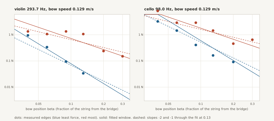
What it found:
- On 12 of the 16 notes (I grouped them by lower-edge slope steeper than -2, after seeing the data) the lower edge falls with
betaat a slope between -2.18 and -2.98, mean -2.61. The upper edge on the same notes has mean slope -1.39. Those two numbers agree with the fitted -2.52 and -1.41, and both are steeper than Schelleng's -2 and -1. - On 4 notes the lower edge barely depends on bow position: violin A4 (-1.14), C5 (-0.52) and E5 (-0.32), and cello E4 (-1.33). Pooling all 16 notes gives -1.77 and -1.20, which looks like a compromise between two behaviours.
- The fit is not good to a factor of 1.35 by this criterion. Of the 69 measured lower edges, 57% fall within a factor of 1.35 of it and 87% within 2. Of the 90 upper edges, 31% and 83%.
- The window depends on the player's help. With
attack_skillat 0, so friction alone starts the stroke, the median measured lower edge is 2.26 times the fit, and only 11% of lower edges fall within 1.35. The fit describes the window for a player who helps a stroke speak. - The four odd notes are not explained by the body. I repeated the sweep on 6 of the notes (four violin, two cello) with bridge coupling at 0 (the bridge does not move, so nothing feeds back). A4 and E5 kept their shallow slopes (-1.17 and -0.13).
- The upper edge is rough. In 65 of the 96 sweeps the set of good forces broke into more than one run, so "the most force that works" is less crisp than the diagram makes it look.
Schelleng's formulas also differ from the fit in the exponents on impedance and speed. The fitted lower edge goes as Z^1.23 v^1.46 and the upper as Z^1.18 v^1.15 (schelleng_window in engine.rs), against Z^2 v and Z v. The model has no free parameter for the bridge resistance R; the body supplies it. I expect it to vary with frequency around each body mode, but I did not measure it.
I stopped here on purpose. The model disagrees with the textbook slopes in a consistent direction on most notes, by a stated amount, and disagrees with itself on four notes for a reason I have not found. The view's diagram is an estimate; the sound is always the simulation. I expect the four notes to be worth a closer look before anyone builds on the fit.
5. The body
body.rs splits the body by job.
The coupled modes are the ten strong low ones: the air mode A0, the corpus modes around 400 to 600 Hz, and the bridge hill at 2.6 kHz. They run at the string rate. Their summed velocity is the bridge's motion, and it is fed straight back into every string's bridge reflection:
let bridge_ref = -self.g_bridge * self.bridge_lp.process(x, self.bridge_a) + bridge_velocity;The engine loop is a two-way exchange:
let v_bridge = self.body.bridge_velocity;
for s in 0..n_all {
    // ...
    total += self.strings[s].tick(ex, v_bridge, glide);
}
let (l, r) = self.body.tick_coupled(total);
Every string sees the bridge as the other strings and the body left it. That feedback is what gives each note a slightly different decay and colour depending on where it falls against a body resonance, lets open strings ring in sympathy, and, pushed hard, makes a wolf note. The bridge velocity passes through a soft ceiling, 0.5 * tanh(2 v), so extreme settings cannot run away.
The radiating modes are 40 more, log-spaced from about 1.1 kHz to 10 kHz with jitter and a per-mode gain scatter. They are driven by the bridge force but do not push back, so they run at the base rate. A seed picks the field, so a different seed is a different maker's instrument of the same family. They pan into two virtual microphones.
Every mode is a two-pole resonator, the velocity response of a damped mass and spring. Frequencies at size 1 (A0 275 Hz, CBR 405, B1- 470, B1+ 540) are figures commonly quoted in violin-acoustics surveys, used as illustrative defaults. They are not a measurement of one instrument. Every frequency scales with 1 / size, except the bridge hill, which scales with the square root, because a bass bridge is not four times a violin's in every dimension.
Evidence
- With the body on, the mean change in harmonic balance across the first 16 harmonics is 4.2 dB against the bare bridge force, and the level rises from -21.1 to -15.0 dBFS. The body reshapes the sound.
- The size axis moves the modes as designed: A0 sits at 279 Hz on the default body, 233 Hz at size 0.13 (a viola), 103 Hz at 0.72 (a cello) and 70 Hz at 1.0 (a bass). The bridge hill goes 2622, 2396, 1592 and 1311 Hz on the same four bodies.
- No coupling means no sympathy. Bowing G4 on the D string with the bridge coupling at 0 leaves the open G string exactly silent (level 0.000). At the normal 0.35 it rings at 0.115, and at 0.9 at 0.323. The levels are the string's own running amplitude estimate, in arbitrary units.
I chose hand-picked coupled modes over a measured body for one reason: a measured body tells you what one violin does, and the instrument laboratory below needs every mode to move with a knob.
6. The virtual player
A bowed note is not a note-on. The player in engine.rs decides what a violinist's hands would do:
- String choice. The highest open string at or below the pitch. If that string is held, the next one down that can reach it, so a second note that arrives with the first is a double stop.
- Chord or slur. Notes starting within 40 ms of a held note form a chord. Later ones slur, with the bow carrying on and the finger sliding.
- Bow reversal. A new stroke on a releasing string reverses the bow.
- Intonation by ear. While a stopped string is in Helmholtz motion, the player compares the period it is actually vibrating at with the one the note wants and eases the finger. The pull is clamped to 3%.
- Vibrato with a delayed onset, none on open strings (there is no finger to roll).
- Pizzicato and col legno as short force pulses on the bow point, and a release that either rings on or is stopped by the bow.
- Force scaled per string.
force_centersets what the middle of the force knob means for this string, pitch and speed, so the same knob position is a sensible force on the G string, the E string and a bass. Move the bow toward the bridge and that same setting falls through the lower edge of the window.
The attack
A bowed string does not begin in Helmholtz motion. The first few periods are chaotic, and the string can fall into multiple slipping and stay there. attack_skill is the player's answer. At high skill, for the first few periods the player imposes an ideal stick-slip cycle at the bow (what the code comment calls a perfect attack in Guettler's sense), then hands over to friction. The second half is attack assist: if the string is double-slipping although the asked-for force is inside the window, the player leans in until it speaks and then eases off.
strings_behaviour_report measures the time until one release per period holds for ten periods:
| Note | Skill 0 (friction alone) | Skill 0.9 (default) | Skill 1.0 |
|---|---|---|---|
| Violin G3 | never (raucous, 2.00 slips per period) | 0.045 s | 0.055 s |
| Violin A4 | 0.179 s | 0.013 s | 0.013 s |
| Violin B5 | 0.155 s | 0.006 s | 0.010 s |
| Cello C2 | 0.667 s | 0.197 s | 0.258 s |
| Bass E1 | 1.132 s | 0.580 s | never (raucous, 2.96 slips per period) |
Two results are worth reading twice. Without the guide, a bare-friction start on the violin's G string never settles in this render. And more skill is not always better: the bass E1 speaks at 0.9 and fails at 1.0. I have not traced the second one. The default is 0.9.
7. The instrument laboratory
Every physical dimension is a continuous control. body_size runs from -1 to 2.5 as a power of four on the frequency divisor, so 0 is a violin body, about 0.13 a viola, 0.72 a cello, 1 a bass, 2.5 a divisor of 32. With "tuning follows size" on, the open-string tuning is interpolated in pitch along the same axis, so a slider takes the instrument from violin to viola to cello to bass and beyond. String mass changes impedance, stiffness the inharmonicity, rosin the friction curve, bow grit the hair noise. Up to six unbowed strings ring in sympathy. The DAW ships a Hardanger fiddle, which is a real if rare instrument with understrings, and three invented presets: glass violin, octobass and wolf cello.
Measured behaviours:
- The wolf. Cello at 163.6 Hz, bridge coupling 1.0. At force knob 0.3 the string double-slips (2.00 slips per period) and the measured pitch is 1200 cents up, an octave above the note; the level is -28.1 dBFS. At force 0.7, Helmholtz motion (0.99 slips per period, 0.0 cents off, -3.5 dBFS). On a normally coupled cello (coupling 0.35) the same light bow at 0.3 plays that note cleanly (0.99, -17.9 dBFS). The wolf appears with strong coupling and goes away with a firmer bow.
- Sympathy. Bowing G4 makes the open G string ring 24.2 times as strongly as bowing F#4 does. A sympathetic string tuned to 440 Hz rings at 22.2 times the level of one tuned to 415.3 Hz while A4 is bowed.
- Impossible instruments stay bounded. The report renders 108 instruments built from the extremes of body size, force, speed, bow position, string mass, coupling and stiffness. Every sample is finite, and the largest is 1.000, which is the output stage's soft knee doing its job.
8. Physics View and one held note
The audio model and the picture do not run at the same rate. PhysModVoice publishes into PhysModShared every 512 output samples, about 86 times a second, through atomics: string frequency, bow position, force and speed, the Schelleng window edges, stick fraction and slips per period, 64 points of each string's displacement, and the ten body modes. The widget in widgets_physmod.rs reads that state and draws it. The audio thread never takes a lock.
The string's shape is rebuilt from the travelling waves. Along a string the slope is (v- - v+) / c, so integrating the difference of the two velocity waves along the delay lines gives the displacement, pinned to zero at both ends. That is the picture from the textbooks, drawn from the simulation's own state.
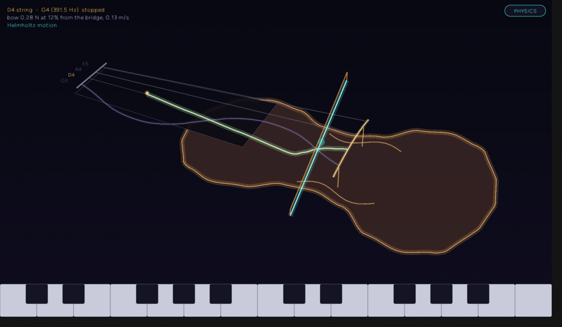
Turning on Physics View adds what is normally invisible:
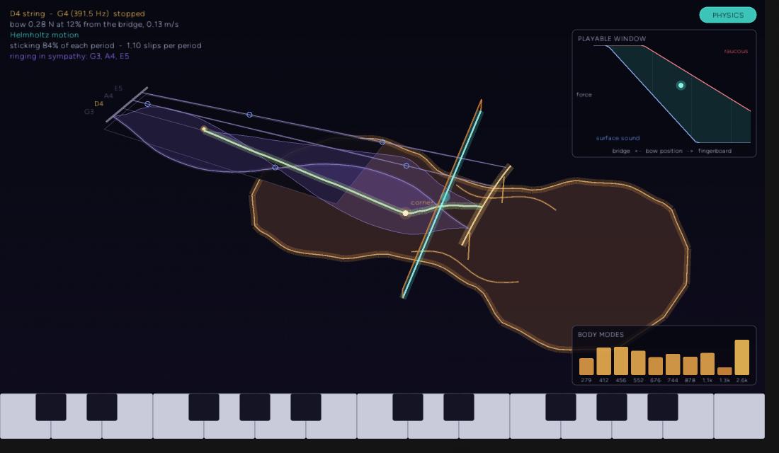
The readout in the corner is the shared state at the moment the test took the picture: 0.28 N at 12% from the bridge, 0.13 m/s, 84% of each period stuck, 1.10 slips per period, ringing in sympathy on G3, A4 and E5. The dot in the diagram sits between the two edges. The body-mode bars along the bottom are the ten coupled modes' current levels.
A cello with sympathetic strings shows the same thing at a different scale:
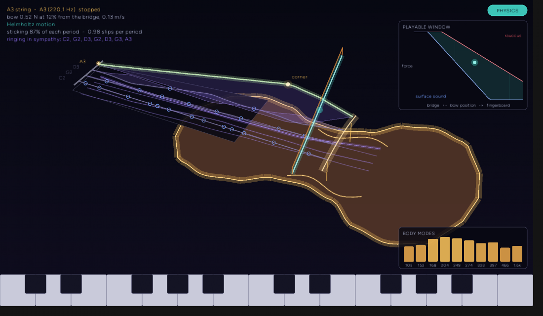
The pictures come from tests/physmod_view.rs, which drives the real widget with a real PhysModVoice and rasterizes on the CPU. The five view tests pass; they cover the drawing, the Physics View overlay, the chip click, a drag in the playable-window diagram moving the bow, and the sympathetic strings.
This is the "one instrument, two representations" pattern the later posts reuse. A bow drag in the 3D view, a drag in the diagram, the knobs, the AI tool and automation all move the same held note, through the four atomics in PhysModLive (force, speed, position, vibrato depth). The view never invents a relationship the sound does not have: what it draws is what the model published.
9. In the DAW
A synth track with waveform physmod gets a PhysModInstrumentVoice, one live instrument per track, with notes sent to it through a command queue so that they share strings and a body. That sharing is what makes a slur or a double stop possible. daw_physmod.ts holds the presets, settings and the laboratory controls, and registers the daw_physmod tool. Its hear action returns the analysis: note, pitch in Hz, cents off, level and brightness. Offline export runs the same notes through render_performance.
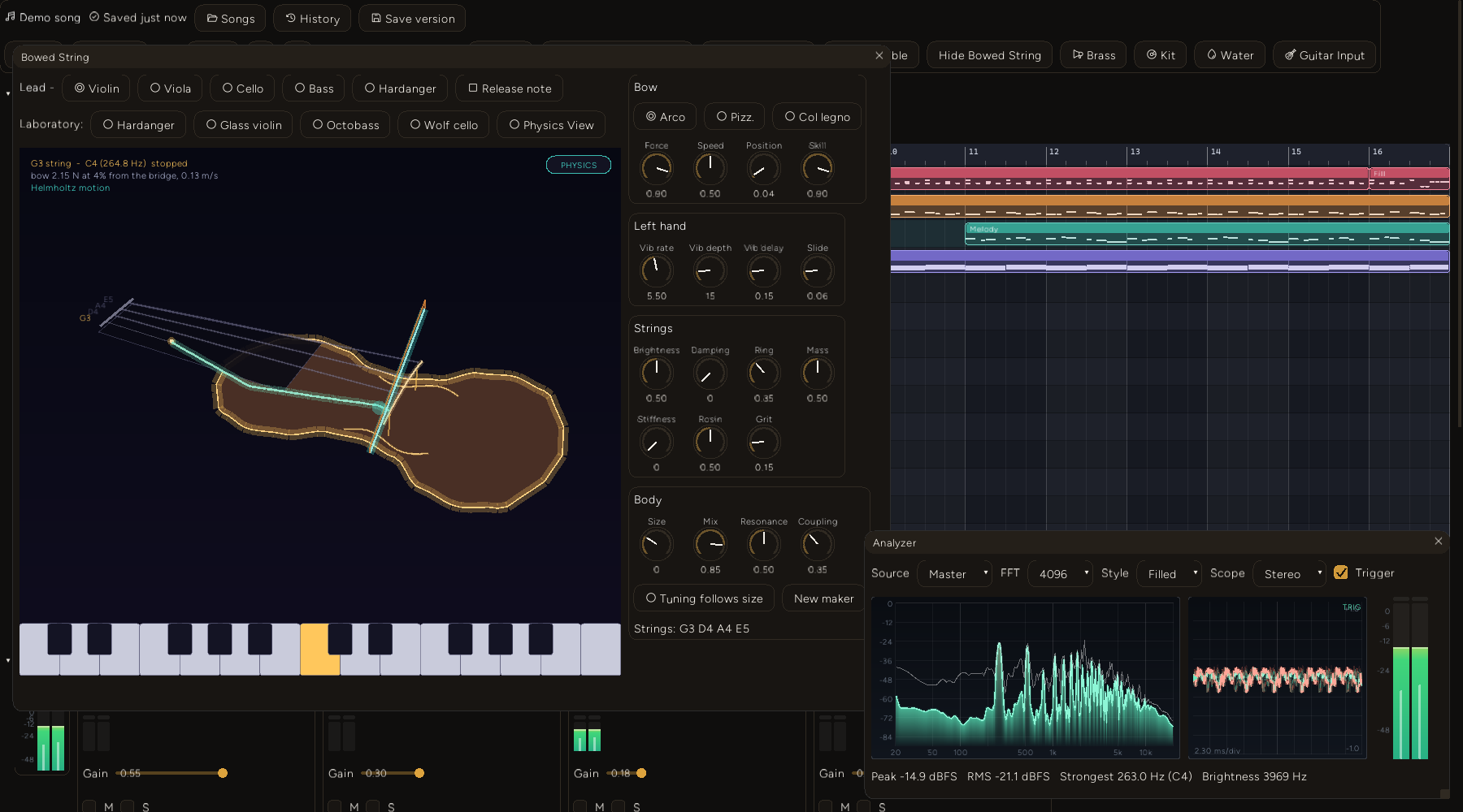
That picture is from tests/daw_physmod_live.rs: a real DAW window, a held C4 on the track bus, a release, a latched note brightening as bow force goes from 0.1 to 0.95 (the analyzer's brightness read 1709 Hz, then 3517 Hz), a bow drag while sounding, violin and cello on the same note, and a song playing through the track. The run passed in 12.07 s and wrote seven PNGs. The events were injected by the test driver, not a musician's hand.
Cost. strings_cost_report renders 10 seconds of audio through Engine::next_frame and divides the wall time by the audio time. Median of three runs, release, i5-12500, single thread, engine only (no voice wrapper, no publishing, no mixing):
| Case | Share of one core |
|---|---|
| One bowed note | 2.0% |
| Four strings bowed at once | 2.2% |
| One note, four sympathetic strings | 3.1% |
| One note, six sympathetic strings | 3.7% |
| Cello, one note | 2.0% |
| Bass, one note | 2.0% |
A whole instrument is about 2%, and each sympathetic string adds about 0.3 percentage points. That is lower than the figure the design doc carried, 4% plus 1% per string, which I did not reproduce. I did not measure inside the running DAW.
10. How this was verified without listening
The instrument was built and tuned without anyone listening to it. Each behaviour was measured from rendered audio, and the tests keep the measurements in place. The table gives the claim and the test that holds it. Results are from this run.
| Claim | Where | Result |
|---|---|---|
| Bowed notes in tune, violin within 6 cents, cello within 8, bass within 10 | physmod::tests (unit), physmod_synth.feature | Pass |
| A normal stroke is Helmholtz motion: one release per period, stuck about 1 - beta, settles in under 0.2 s | same | Pass |
| Too little force near the bridge gives surface sound; a firm bow cures it | same | Pass |
The lower force edge rises far faster than 1 / beta | physmod::tests | Pass (ratio over 3.5) |
| Faster bow is louder (about 6 dB per doubling); ponticello is brighter than tasto | same | Pass |
| The open G rings for a G and not for an F sharp; coupling controls how much | same | Pass |
| A wolf on a strongly coupled cello, tamed by a firmer bow, absent at normal coupling | physmod_synth.feature | Pass |
| Pizzicato decays; stiffness stretches partials; output is bounded for impossible instruments | physmod::tests | Pass |
| The view draws the instrument, Physics View overlays, chip and diagram interactions | tests/physmod_view.rs | 5 of 5 |
| No allocation on the audio thread while notes arrive, slur and release | tests/physmod_no_alloc.rs | Pass |
| Settings, presets, morph and repair of old songs | tests/daw_physmod.test.ts | 10 of 10 |
Counts from this run:
cargo test --release --lib physmod: 41 passed, 0 failed. The filter also matches the friction, DSP and widget unit tests.cargo test --release --test physmod_synth_bdd: 24 scenarios, 151 steps, all passed.physmod_view: 5 passed.physmod_no_alloc: 1 passed.daw_physmod.test.ts: 10 passed.
The no-allocation test installs a counting global allocator that watches only the thread pulling samples. Another thread sends a phrase of notes with slurs, a double stop, pizzicato and live bow moves while the audio side runs three seconds of samples. The count must be zero. Sample-by-sample tests catch wrong values; this one catches a Vec::push in the middle of the audio callback.
The earlier post flagged two tests whose names promised more than they measured (a pitch test named for the strongest partial and a damping test that only compared a fixed release). The rewritten feature file contains neither.
11. Decision log
Waveguide over modal or finite-difference strings. A waveguide gives you the bow as a point where two delay lines meet, which is the structure the friction law wants. I did not build the alternatives, so this is a reason and not a comparison. The cost I did hit is fractional-delay error and the termination filters, which is why tuning is solved from the sum of every delay in the loop.
Friction solved in closed form, not iterated. The hyperbolic curve makes the slip solution a quadratic, so the solve is a square root. I did not try iterating.
Four delay lines, not one folded loop. The earlier voice regenerated its own signal because a friction-like pull in a single folded loop settled at a fixed point instead of oscillating. Splitting the string at the bow gives the friction law two segments to act between, which is why there are four delay lines and not one.
Hand-picked coupled modes. Discussed above. A measured body would sound like one instrument and could not be scaled to a bass or an octobass with one knob.
Two body rates. The ten coupled modes run at 88.2 kHz because they feed the strings back. The 40 radiating modes run at 44.1 kHz because they do not push back, which is the source comment's reasoning. I did not measure running all fifty at the string rate.
A player, not just a synth. Note-on with a velocity is not what a bowed instrument does. Without the guided attack, the violin's G string never settles in the report above. With it, the settle time on the violin is under 50 ms. The tradeoff is that some of the "Helmholtz window" the fit describes is the player's, not the physics'.
Fit the window to the model. I fitted schelleng_window to the sweeps of the model, not to Schelleng's formulas, so the view's diagram matches what the sound does. The tradeoff, shown in section 4, is that the fit is rougher than its comment says and tracks four notes badly.
12. Failure notes and known limits
Failure notes
- The stiffness knob saturates on low notes, described in section 2. The solver's cap on allpass delay is the reason. Nothing warns you.
attack_skillat 1.0 fails to start a bass E1 in this render (never settles, 2.96 slips per period), while 0.9 works. Skill 0 fails on the violin's G string.- The Schelleng fit disagrees with its own sweep on four notes and is looser than its comment says (section 4). The cause is not the bridge.
- The live DAW test failed at first for a stale reason: its analysis call read a field named
strongestHz, and the tool now returnspitchHzandcentsOff. I renamed the three references intests/daw_physmod_live.rs. Its pitch assertion, a 10% tolerance, is loose enough that the cello's A3 at 209.2 Hz against 220 passes; it is a smoke test, not a tuning test. - A note on tooling:
PhysModParamshas two arrays whose lengths are written as literals because a named constant there makes rustc 1.94 hit an internal compiler error whenever a caller builds the struct with..baseinside a closure. The code asserts the literals still match the constants.
Known limits
- The bottom of the bass takes 0.3 to 0.6 s to speak: E1 0.58 s, A1 0.34 s, in this run.
- Not modelled: bow width, torsional waves, thermal (temperature-dependent) friction, the string's second polarisation.
- The friction is the speed-only hyperbolic curve. I did not test the thermal model.
- The window fit is an estimate in the view. The sound is always the simulation.
- Manipulating the body, bridge or string construction directly from the 3D view is not built. Those are knobs.
- The body's modes are illustrative, not a measured instrument.
- I did not listen to any of it. Nothing in this post says it sounds like a violin. The claims are pitch, motion, level and spectrum, measured on samples.
What's next
The next post is a tube, a pair of lips and a shock front: brass uses the same "one instrument, two representations" view, and this time the resonator is the whole instrument and the player matters more. The four odd notes in the Schelleng sweep stay open. If they turn out to be a bug, the window fit changes with them.